Introduction

I recently worked on re-factoring code for a QGIS plugin that I use a lot, GarminCustomMaps. This post covers two areas of that work:

1. Image tiling optimization
2. Benchmarking factorization algorithms

1. Image tiling optimization

The GarminCustomMaps plugin for QGIS exports the current map canvas to a .kmz file. These files can then be used in some handheld Garmin devices as “Custom Maps”. One of the limitations of this format is a maximum file size of 1MB for an image that Garmin can draw. In order to ensure that the output .kmz file fits within this constraint, GarminCustomMaps calculates the image size that would result from exporting the current map canvas and provides the option of splitting this image into several contiguous tiles. Garmin devices can load kmz files with multiple tiles, but limits the number of tiles to a maximum of 100 or 500, depending on the model of the device. This functionality gives the user the information and tools needed to ensure their maps will be compatible with Garmin devices.

Dividing an image into several smaller images is called tiling. There are various ways of tiling an image, depending on constraints and other criteria. One of the goals of the re-factor was to write an optimization function that would achieve the required tiling as fast as possible. The criteria chosen were as follows:

• Each tile must be less than a given maximum number of pixels
• Each tile must have an aspect ratio as close to 1:1 as possible
• The coverage of the tiles over the full image extent has as few trailing pixels as possible

It is also required that the total number of tiles is less than the maximum device-supported number of tiles.

To solve this optimization problem we calculate an optimization score for tile dimensions w × h. This calculation is based on the seleted tiling criteria. The maximum score corresponds to the optimal tile size for a given canvas size.

Optimization score

Given a map canvas with extent x × y and a tile with dimensions w × h:

• Tile size \(a = wh\)
• Tile aspect ratio \(s = \frac{min(w,h)}{max(w,h)}\)
• Number of tiles of size \(n = ceil(\frac{x}{w})ceil(\frac{y}{h})\)
• Pixel remainder \(p = an - xy + 1\)

We can then calculate the optimization score: $$ Z = \frac{as}{np}$$

GarminCustomMap is written in Python. To solve the optimization problem in Python, we chose to use numpy. This library for numerical computation offers a powerful data model that is well suited to solving linear algebra problems. In numpy all matrixes are abstracted as arrays. Calculations can be performed on whole arrays, which is faster and more mathematical than looping through lists.

In this article, we will illustrate the development of a fast and efficient algorithm to solve our optimization problem by going through several iterations that each highlights an improvement.

Brute force

The first approach we will examine is least efficient, but most obvious: brute force. We can think of this approach as calculating an optimization score for every possible combination of x × y, then selecting the highest score thereby arriving at the optimal tile size.

To implement this algortihm, we created a solution space mesh using numpy arrays and use the vectorized math of numpy to calculate all possible combinations of tile dimensions for a given canvas extent.

Note: While this article cosiders algorithm development starting with a brute force approach and making incremental changes to improve performance, the even more brute force approach of using nested for loops to solve the whole solution space won’t be considered — this is why we have numpy.

Let’s see how this algorithm looks:

def optimize_bf (x, y, max_tile_size, max_num_tiles):
    """Brute force tiling optimization method"""
    # Set up solution space
    W, H = np.meshgrid(np.arange(1,x+1), np.arange(1,y+1))

    # Tile size
    A = W * H
    # Tile aspect ratio
    S = np.minimum(W,H)/np.maximum(W,H)
    # Number of tiles, rows x columns
    N = np.ceil(x/W) * np.ceil(y/H)
    # Pixel remainder shifted by 1 to avoid division by 0
    P = A * N - img_ext + 1
    # Set score to 0 for tiles that fall outside constraints
    C = (A <= max_tile_size) * (N <= max_num_tiles)

    # Optimization score
    Z = A * S * C / (N * P)

    # Find optimal size
    opt_tile_size = np.unravel_index(np.argmax(Z), Z.shape)
    return (W[opt_tile_size], H[opt_tile_size])

As you can see, moving from a mathematical formulation of a problem to its implementation in numpy is very direct: a powerful paradigm.

How does this code perform?

Let’s examine this figure. On the left we have information about our solution variables, image extent and maximum tile size, the time it took to find the solution, and the optimization results. On the right and in the middle we have two plots showing the same information: the complete solution space and the calculated optimization score. Finally, in the bottom right we have a schematic showing what the tiling would look like with the given image extent and optimized tile size.

Note: Code to generate these plots can be found in the tiling optimization repository that contains all the code in this case study.

Back to the results themselves: our algorithm works fine for small image sizes (less than a millisecond to find a solution!), but what happens if we increase the canvas extent to something realistic, for example a standard screen size 1920x1080 and a maximum tile size of 1024x1024, which will get us close to a 1MB JPEG.

Although this is still OK for practical purposes, memory usage shoots up (this is not represented in the figure).

As we get to larger extents, both CPU and memory usage increases and if we get close to our available RAM the OS just kills the process altogether without Python even being able to throw an exception. Not good. This algorithm does not scale well and is very wasteful.

So how do we improve this code? From the examples above, consider how much of the solution space is just zeros. We don’t need to run calculations for these values, because we know, based on our constraints, that the optimization score will be 0. Also, since numpy defaults to 64-bit floats, we are filling up big chunks of memory.

Let’s think about our actual memory requirements based on the problem constraints and see if we can cut down on memory usage in our algorithm.

dtypes and boolean indexing

Firstly, based on our definitions, only the optimization score Z and tile aspect ratio S arrays are floating point; all our other variables are integer values.

• A is the tile size, and can be at most x × y (the image extent)
• N is the number of tiles for size A, and can also be at most x × y (1×1 tile)
• P is always < A
• S is always between 0 and 1

Let’s look at available data types for numpy arrays:

int16 has a range of −32,768 to 32,767, taking the square root of the maximum, we get a maximum side size of 181 (for a 1:1 aspect ratio tile — a square). Since we are working with images on modern high resolution computer screens, this is probably too small for our needs.

Next we have int32, which is a signed integer with a range of −2,147,483,648 to 2,147,483,647 taking the square root, we have a limit of 46340. Much better. If we want to give ourselves a bit more overhead, we can use the unsigned version, which will allow us work with values of 0 to 4,294,967,295.

For floating point values, we likewise have float16 and float32. float16 is a bit small for our needs, and may lead to overflow errors while calculating the optimization score; we will use float32.

Let’s change our function:

def optimize_dtb (x, y, max_tile_size, max_num_tiles):
    W, H = np.meshgrid(
                       np.arange(1,x+1, dtype=np.uint32),
                       np.arange(1,y+1, dtype=np.uint32))
    Z = np.zeros((y, x), dtype=np.float32)
    img_ext = x*y

    # Tile size
    A = W*H
    # Calculate the side ratio
    S = (np.minimum(W,H)/np.maximum(W,H)).astype(np.float32)
    # Number of tiles, rows x columns
    N = (np.ceil(x/W) * np.ceil(y/H)).astype(np.uint32)
    # Pixel remainder shifted by 1 to avoid division by 0
    P = A*N - img_ext + 1
    # Mask the values that fall outside the constraints
    m = (A <= max_tile_size) & (N <= max_num_tiles)

    # Optimization score
    Z[m] = A[m] * S[m] / (N[m] * P[m])

    # Find optimal size
    opt_tile_size = np.unravel_index(np.argmax(Z), Z.shape)

    return (W[opt_tile_size], H[opt_tile_size])

Notice our optimization score calculation uses an indexed version of each array. Compared to the brute force method, where we were setting values that fall outside our constraints to zero after performing our calculation, in this case we are make the code more efficient by constraining calculations to values of interest only. In python this is called boolean indexing. Boolean indexing is done by assigning a True value to locations where we want a solution, and False everywhere else, in an array that has the same shape as the inputs. This array is then used to mask the solution space, reducing the number of required calculations.

Let’s see how the two improvements made to our code impact performance. We will use the same examples as above.

So not much of a difference at these sizes. But let’s try a much larger solution space (no visualization this time):

[esan@mwork tiling_optimization]$ python optimization.py
Image extent: 36000000 (6000 x 6000)
Maximum tile size: 1048576

A = tile size
S = ratio of tile sides (always < 1)
N = number of tiles
P = pixel remainder
Optimization score: Z = AS/NP
Optimization fuction: bf

Calculation time: 13.31 s

Optimal tile size: 1000 x 1000
Pixel remainder: 0.0

and

[esan@mwork tiling_optimization]$ python optimization.py
Image extent: 36000000 (6000 x 6000)
Maximum tile size: 1048576

A = tile size
S = ratio of tile sides (always < 1)
N = number of tiles
P = pixel remainder
Optimization score: Z = AS/NP
Optimization fuction: dtb

Calculation time: 8.004 s

Optimal tile size: 1000 x 1000
Pixel remainder: 0

Note: There is another mechanism available in numpy for excluding some elements of an array from calculations: using masked arrays. After some testing I found that the masked method is slower than boolean indexing. As hinited at in the documentation, masked arrays really do seem to be mainly useful for dealing with NAN and other invalid data, rather than a way to speed up calculation.

So we’ve achieved noticeable improvement, and are able to process potential canvas sizes of any practical extent. But can we do better?

Let’s recall that one of our criteria for selecting the optimal tile size is the pixel remainder — we want the coverage of the original image extent to have as few trailing pixels as possible. Ideally, we select a tile size such that the tiling perfectly covers the original image.

With this in mind, we can change our algorithm to start with a much smaller solution space than a mesh of all possible combinations.

Factors method

If the original image extent dimensions can have a perfect solution, the optimal tile size will have sides that are factors of those dimensions. If we find all the factors of the x and y extent of the original image, we need to solve the optimization for this subset of the solution space only. If the image dimensions are prime, then we can fall back to the dtb method.

So with this approach, our optimization score algorithm doesn’t change. What changes is that we add a step to find our factors solution space by a process called factorization.

Factorization is a well studied problem in mathematics because factors are useful for many areas, including cryptography. Several factorization algorithms exist. For our purposes, we will compare two of the simpler algorithms and choose the faster one.

2. Benchmarking Factorization Algorithms

The first algorithm is brute force.

def factors_all (n):
    '''This is a brute force algorithm that returns a list of all factors of n
    including 1 and n. We cycle through all numbers from 1 to n and see
    if they divide n evenly.
    '''
    a = []
    for i in range(1, n+1):
        if n % i == 0: a.append(i)
    return a

This method is self explanatory and returns a nicely sorted list of all divisors of n — exactly what we need to create our reduced solution space.

The second algorithm is called trial division.

import numpy as np
from itertools import combinations

def factors_trial_np (n):
    '''This trial division factorization algorithm is taken from Wikipedia:
    https://en.wikipedia.org/wiki/Trial_division
    Additional lines use the factorization to get all factors of n including
    1 and n.
    '''
    a = []
    while n % 2 == 0:
        a.append(2)
        n //= 2
    f = 3
    while f * f <= n:
        if n % f == 0:
            a.append(f)
            n //= f
        else:
            f += 2
    if n != 1: a.append(n)

    b = []
    for i in range(1, len(a)+1):
        b += [np.prod(x) for x in combinations(a,i)]
    b = [*set(b), ]
    b.append(1)
    b.sort()
    return b

The vanilla trial division algorithm returns a list of prime factors of n, but since we need a list of all divisors of n, we added several additional lines.

for i in range(1, len(a)+1):
    b += [np.prod(x) for x in combinations(a,i)]

Here we use the combinations method from the itertools module to get all the products of all combinations of length i of a list a. This gives us a none-sorted and none-unique list of all divisors for n.

We then take only the unique values and sort them:

b = [*set(b), ]
b.append(1)
b.sort()

Timing

We can use the timeit module to benchmark these two algorithms. timeit runs a function repeatedly and returns the average runtime. We want to run the benchmark for several input values to get a sense of how the algorithms scale. To achieve these two goals and maintain readability of the code, we will use a decorator to wrap our factorization functions with some timeit constructs.

import timeit
from functools import wraps

def run_timeit (func):
    @wraps(func)
    def wrapper_timeit (s):
        return timeit.timeit(lambda: func(s), number = 100)
    return wrapper_timeit

For a great resource on wrappers see this article on Real Python

While not strictly speaking required, the @wraps(func) line is key. This use case is a great example of why that decorator should almost always be used when writing your own decorators. Since we are passing the function by reference to the Pool.map() (see next section) method, the decorated reference should be resolved to our actual factorization function, rather than the wrapper_timeit.

A good explanation of the problems I was running into before adding that line can be found here.

Here’s what running the above code without @wraps(func) looks like:

Traceback (most recent call last):
  File "/home/esan/src/projects/testing/factors_comparison.py", line 69, in <module>
    y_all = p.map (factors_all, x)
  File "/usr/lib/python3.10/multiprocessing/pool.py", line 364, in map
    return self._map_async(func, iterable, mapstar, chunksize).get()
  File "/usr/lib/python3.10/multiprocessing/pool.py", line 771, in get
    raise self._value
  File "/usr/lib/python3.10/multiprocessing/pool.py", line 537, in _handle_tasks
    put(task)
  File "/usr/lib/python3.10/multiprocessing/connection.py", line 211, in send
    self._send_bytes(_ForkingPickler.dumps(obj))
  File "/usr/lib/python3.10/multiprocessing/reduction.py", line 51, in dumps
    cls(buf, protocol).dump(obj)
AttributeError: Can't pickle local object 'run_timeit.<locals>.wrapper_timeit''

Benchmarking

We are now ready to run the benchmark and plot the results.

import numpy as np
import matplotlib.pyplot as plt
from multiprocessing import Pool

if __name__ == '__main__':
    # Set up logarithmic sample space
    # 50 evenly spaced samples in a log space from 1 to 2^15
    n = 15
    x = np.logspace(1, n, num=50, base=2, dtype=np.uint32)

    # Run both algorithms in a process pool and time
    with Pool() as p:
        y_all = p.map (factors_all, x)
    with Pool() as p:
        y_trial_np = p.map (factors_trial_np, x)

    # Plot results
    fig, ax = plt.subplots (layout='tight')
    ax.loglog (x, y_all, marker = '.', label='brute force division')
    ax.loglog (x, y_trial_np, marker = '.', label='trial division (numpy)')
    ax.set_xlabel ('number to factor')
    ax.set_ylabel ('average loop time [s]')
    ax.set_title ('Benchmarking factorization algorithms')
    ax.legend ()
    ax.grid(True)
    plt.show ()

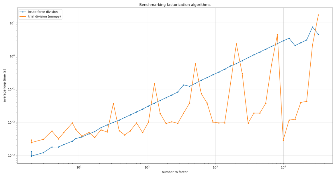
Admittedly, this result was very confusing. After some poking around, I tried using the math module’s prod() function instead of the one from numpy. It made a huge difference. Maybe the slowdown is because numpy needs ndarray inputs, where math can handle any iterable?

Let’s change our factorization function from this:

for i in range(1, len(a)+1):
    b += [np.prod(x) for x in combinations(a,i)]

to this:

for i in range(1, len(a)+1):
    b += [math.prod(x) for x in combinations(a,i)]

and add additional plotting axes:

with Pool() as p:
    y_trial_math = p.map (factors_trial_math, x)
ax.loglog (x, y_trial_math, marker = '.', label='trial division (math)')

And here’s what we get:

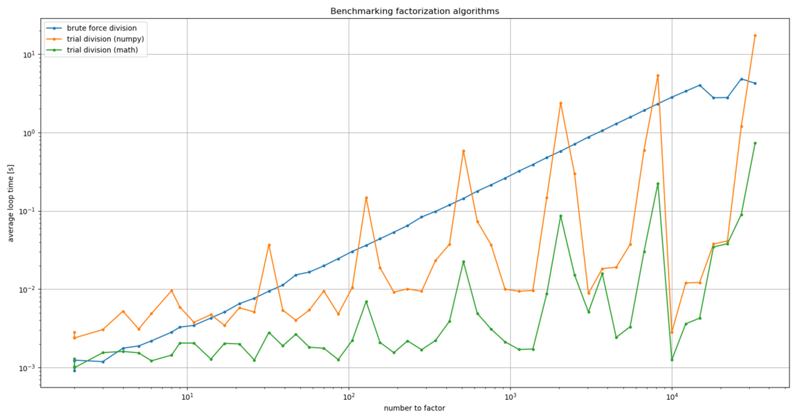
Much better!

Conclusion

We have developed a fast and efficient factorization algorithm that we can use to reduce our required solution space in the optimization problem.

Note: There are other, more efficient, factorization algorithms available that should be considered and implemented. We will leave this for future work. For our solution space requirements, we can get a reduced solution space in less than a second for some of the largest extents we can expect to see.

Optimization score revisited

We now have the necessary element for the factors optimization method. Nothing changes in the optimization calculation score itself. The only change we need to make is setting up the solution space:

def optimize_fac (x, y, max_tile_size, max_num_tiles):
    '''Factors optimization method for finding solutions with
    perfect coverage.
    '''
    # Get all the factors of x and y
    w = np.array (trial_division (x), dtype=np.uint32)
    h = np.array (trial_division (y), dtype=np.uint32)

    # Set up solution space
    W, H = np.meshgrid (w, h)
    Z = np.zeros_like(W, dtype=np.float32)

The rest is the same as optimize_dtb above.

3. Implementation for GarminCustomMaps plugin

We’ve covered a lot: we developed an efficient and fast optimization algorithm, and we’ve found a fast factorization algorithm that will provide a significantly reduced solution space for extents that are not prime.

The only thing that remains is to implement this code in our plugin.

To make the code clean and maintainable, we will create a new module to keep the factorization and optimization methods. We will then import this module from the main GarminCustomMaps code.

The final implementation can be found here.

Appendix A: Another way of using timeit

In testing out the masked arrays functionality of numpy, I tested the speed of the same code but with masked arrays in one case, and boolean indexing in the other.

Below is a demo of using timeit from the commandline, with short snippets of code stored in text files for setup and the actual code of interest.

This code can be found in the tiling optimization repository

[esan@mwork tiling_optimization]$ cat ti_setup ti_code_masked ti_code_bool
#------------#
# Set up variables and modules
import numpy as np
import numpy.ma as ma
x,y = 5000,6000
img_ext = x*y
max_tile_size = 1024*1024
max_num_tiles = 100
#------------#
#------------#
W, H = np.meshgrid(np.arange(1,x+1), np.arange(1,y+1))
a = W*H
N = np.ceil(x/W) * np.ceil(y/H)
S = np.minimum(W,H)/np.maximum(W,H)
A = ma.masked_where(np.logical_or(a>max_tile_size, N>max_num_tiles), a)
Z = A * S / N
#------------#
#------------#
W, H = np.meshgrid(np.arange(1,x+1), np.arange(1,y+1))
Z = np.zeros((y,x))
A = W*H
N = np.ceil(x/W) * np.ceil(y/H)
S = np.minimum(W,H)/np.maximum(W,H)
m = (A <= max_tile_size) & (N <= max_num_tiles)
Z[m] = A[m] * S[m] / N[m]
#------------#
[esan@mwork tiling_optimization]$ python -m timeit -n 50 -s "$(<ti_setup)" "$(<ti_code_masked)"
50 loops, best of 5: 1.61 sec per loop
[esan@mwork tiling_optimization]$ python -m timeit -n 50 -s "$(<ti_setup)" "$(<ti_code_bool)"
50 loops, best of 5: 840 msec per loop

Appendix B: dtypes overflow

I was a bit ambitious about reducing the memory footprint and got snagged several times in my attempt to cut down memory usage. One of the issues that took me some time to troubleshoot was that the optimization score didn’t always fit into float16:

>>> Z[m] = A[m]*S[m]/N[m]
>>> Z[m]
array([1.878e+00, 2.885e+00, 4.984e+00, 7.512e+00, 1.502e+01, 1.154e+01,
       2.308e+01, 1.691e+01, 2.534e+01, 5.069e+01, 2.597e+01, 3.894e+01,
       7.788e+01, 5.869e+01, 7.825e+01, 1.174e+02, 2.348e+02, 6.762e+01,
       1.014e+02, 1.352e+02, 2.028e+02, 4.055e+02, 1.039e+02, 1.558e+02,
       2.078e+02, 3.115e+02, 6.230e+02, 2.281e+02, 3.422e+02, 4.562e+02,
       6.845e+02, 1.369e+03, 3.130e+02, 4.695e+02, 6.260e+02, 9.390e+02,
       1.878e+03, 1.774e+02, 1.056e+03, 1.584e+03, 2.112e+03, 3.168e+03,
       6.336e+03, 2.129e+02, 1.703e+03, 2.738e+03, 3.650e+03, 5.476e+03,
       1.095e+04, 3.548e+02, 2.838e+03, 9.576e+03, 1.690e+04, 2.534e+04,
       5.069e+04, 5.320e+02, 4.256e+03, 1.437e+04, 3.405e+04,       inf,
             inf, 1.064e+03, 8.512e+03, 2.874e+04,       inf,       inf],
      dtype=float16)
>>> Z = np.zeros_like(A, dtype=np.float32)
>>> Z[m] = A[m]*S[m]/N[m]
>>> Z[m]
array([1.87777781e+00, 2.88461542e+00, 4.98461533e+00, 7.51111126e+00,
       1.50222225e+01, 1.15384617e+01, 2.30769234e+01, 1.68999996e+01,
       2.53500004e+01, 5.07000008e+01, 2.59615383e+01, 3.89423065e+01,
       7.78846130e+01, 5.86805573e+01, 7.82407379e+01, 1.17361115e+02,
       2.34722229e+02, 6.75999985e+01, 1.01400002e+02, 1.35199997e+02,
       2.02800003e+02, 4.05600006e+02, 1.03846153e+02, 1.55769226e+02,
       2.07692307e+02, 3.11538452e+02, 6.23076904e+02, 2.28149994e+02,
       3.42225006e+02, 4.56299988e+02, 6.84450012e+02, 1.36890002e+03,
       3.12962952e+02, 4.69444458e+02, 6.25925903e+02, 9.38888916e+02,
       1.87777783e+03, 1.77347229e+02, 1.05625000e+03, 1.58437500e+03,
       2.11250000e+03, 3.16875000e+03, 6.33750000e+03, 2.12816666e+02,
       1.70253333e+03, 2.73780005e+03, 3.65039990e+03, 5.47560010e+03,
       1.09512002e+04, 3.54694458e+02, 2.83755566e+03, 9.57675000e+03,
       1.69000000e+04, 2.53500000e+04, 5.07000000e+04, 5.32041687e+02,
       4.25633350e+03, 1.43651250e+04, 3.40506680e+04, 8.55562500e+04,
       1.71112500e+05, 1.06408337e+03, 8.51266699e+03, 2.87302500e+04,
       6.81013359e+04, 2.29842000e+05], dtype=float32)
>>>

and this is for:

# Set up conditions
x = 1356
y = 1170
max_tile_size = 1024**2
max_num_tiles = 100